Radially-averaged topset slope

The topset slope of fan or delta can be challenging to quantify, due to the axis-symmetric nature of sedimentary fans, and variability in the surface elevation across the fan.

sandplover implements a metric compute_topset_slope to make this easier.

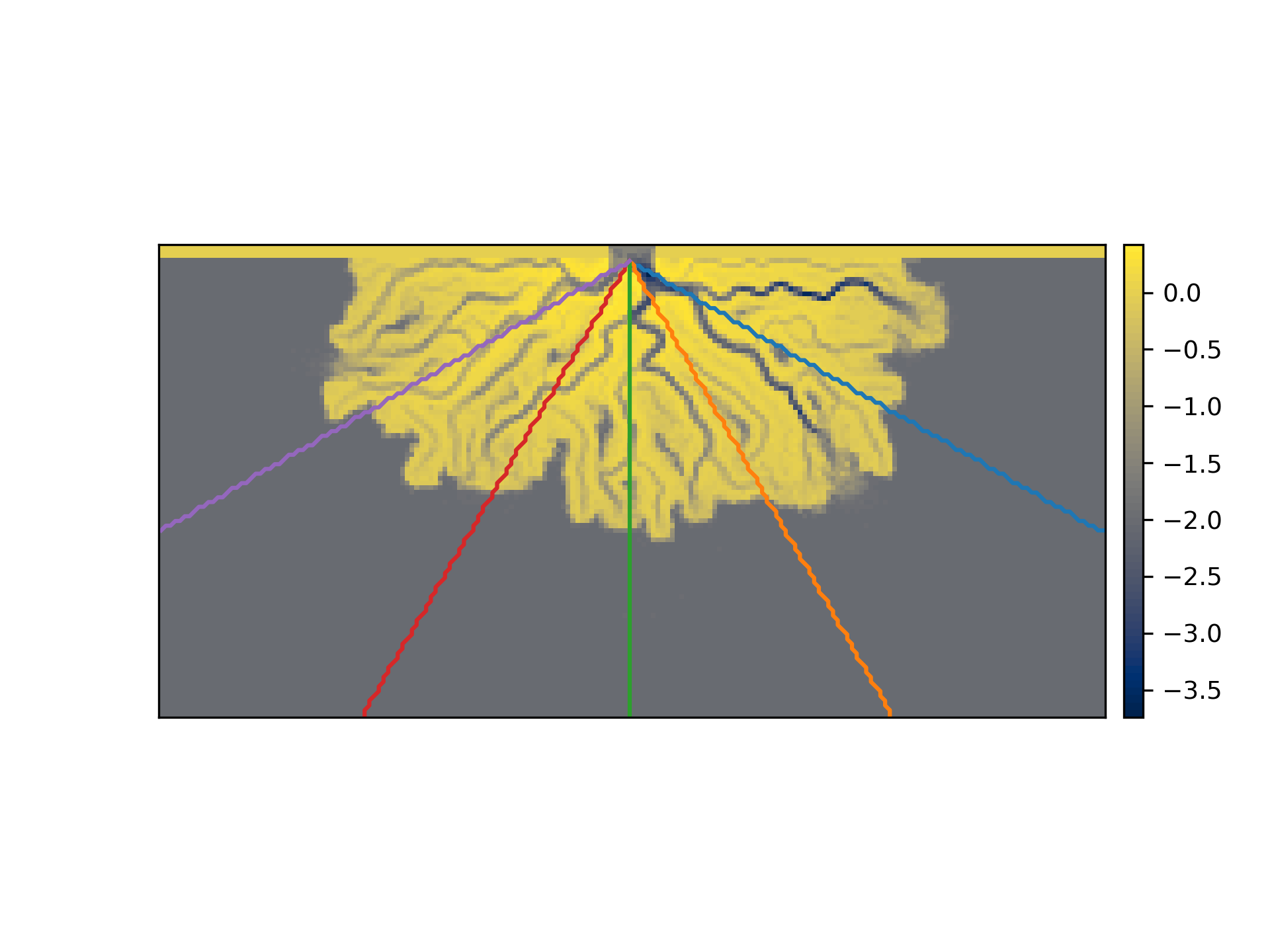
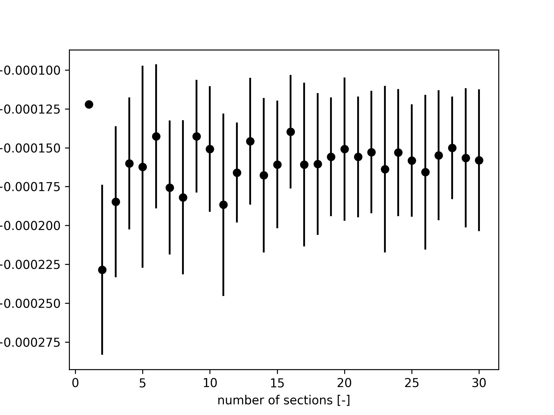
Number of RadialSection

See the effect of an increasing number of RadialSection objects used in the computation.

golf = spl.sample_data.golf()
origin = (
    np.array([golf.meta["L0"].data, golf.meta["CTR"].data]) * golf.meta["dx"].data
)

# make a map with just five sections to see how this would look
from sandplover.plan import _determine_equally_spaced_azimuths
azimuths = _determine_equally_spaced_azimuths(num=5)

fig, ax = plt.subplots()
golf.quick_show("eta", idx=-1)
for a, azimuth in enumerate(azimuths):
    a_section = spl.section.RadialSection(
        golf["eta"][-1, :, :],
        azimuth=azimuth,
        origin=origin,
    )
    a_section.show_trace(ax=ax)

plt.show()

(Source code, png, hires.png)

nums = np.arange(1, 31)
means = np.zeros(len(nums))
stds = np.zeros(len(nums))

for i, num in enumerate(nums):
    means[i], stds[i] = spl.plan.compute_topset_slope(
        golf["eta"][-1, :, :], num=num,
        origin=origin
    )


fig, ax = plt.subplots()
ax.errorbar(nums, means, yerr=stds, marker="none", linestyle="none", color="k")
ax.plot(nums, means, marker="o", linestyle="none", color="k")
ax.set_xlabel('number of sections [-]')
ax.set_ylabel('topset slope [-]')
plt.show()

(Source code, png, hires.png)

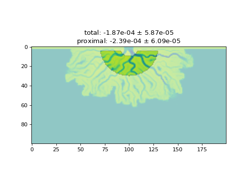
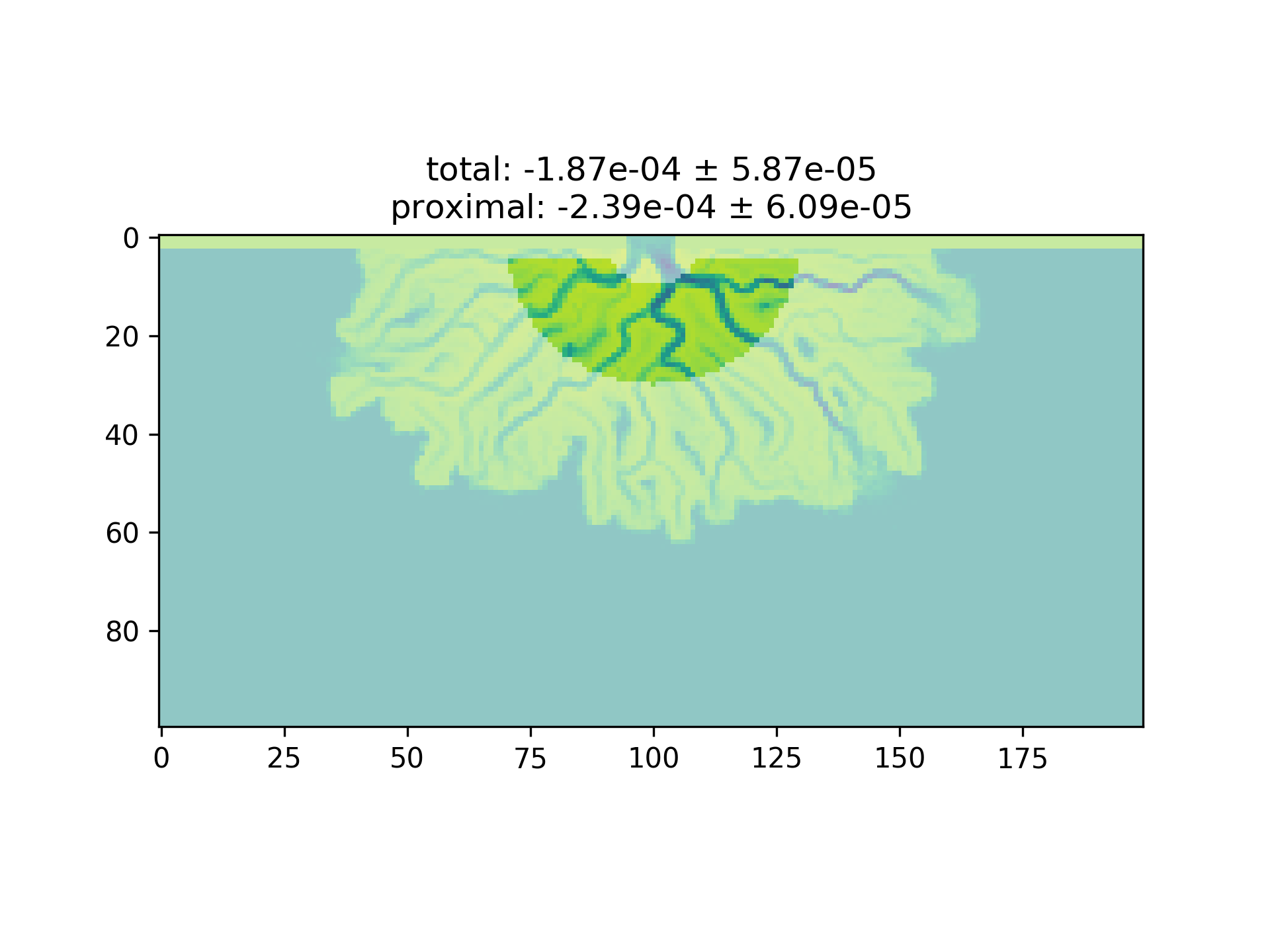
Limit the computation to a proximal region of the delta

# make a copy of the elevation data
elevation = golf["eta"][-1, :, :].copy()

# compute the slope over the full topset
mean_full, std_full = spl.plan.compute_topset_slope(
    elevation, origin=origin
    )

# set up a proximal mask
proximal_mask =  spl.mask.GeometricMask(golf["eta"][-1, :, :])
proximal_mask.circular(rad1=10, rad2=30)
proximal_mask.trim_mask(length=5)

# replace the unmasked data with nan, compute
elevation.data[~proximal_mask.mask] = np.nan
mean_prox, std_prox = spl.plan.compute_topset_slope(
    elevation, origin=origin
    )

fig, ax = plt.subplots()
ax.imshow(golf["eta"][-1], vmin=-5, vmax=1, alpha=0.5)
ax.imshow(elevation, vmin=-5, vmax=1, alpha=1)
ax.set_title(
    f"total: {mean_full:.2e} $\\pm$ {std_full:.2e}\n"
    f"proximal: {mean_prox:.2e} $\\pm$ {std_prox:.2e}"
    )

plt.show()

(Source code, png, hires.png)