Visualization Guide

This guide covers the full range of visualization routines available as part of sandplover, and explains how to create your own visualization routines that build on top of DeltaMetrics.

There are built-in visualization tools in sandplover, which are for the most part attached to the object that you would want to visualize itself. For example, to visualize a section:

spl.section.RadialSection(golfcube, azimuth=70).show("velocity")

There are also built-in visualization style configurations that control the display of certian variables throughout the software. The goal with these style configurations is to reduce the number of steps needed to make visualizations during data analysis and figure production.

This guide is broken into two sections, first explaining these visualization style configurations, then explaining the various built-in methods for displaying data.

Style Configurations

Style configurations for different variables in the underlying data of a Cube are determined by VariableInfo objects that are organized into a dictionary-like VariableSet object. The VariableSet is created during instantiation of every Cube; an existing VariableSet can be provided as an optional argument during Cube instantiation.

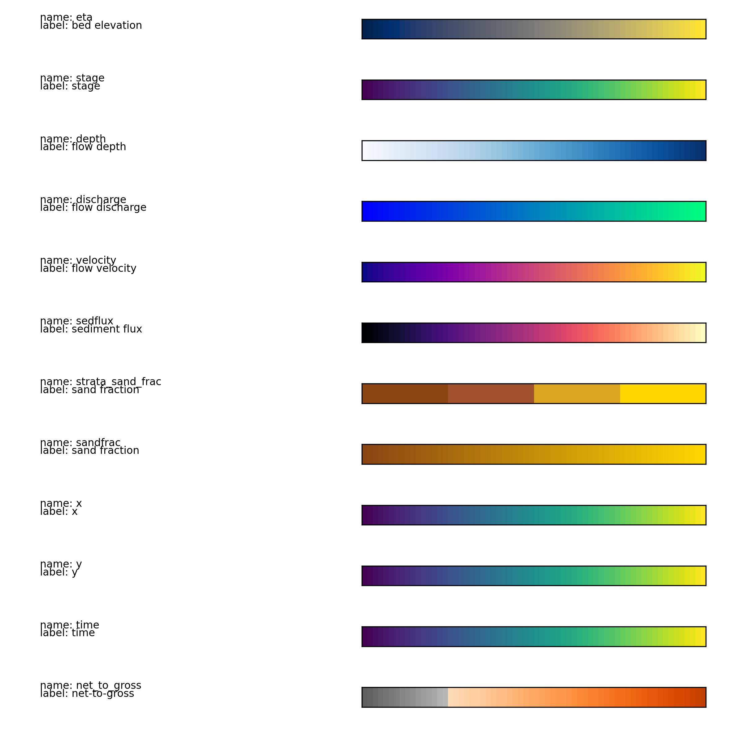
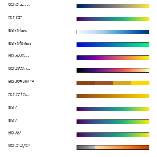
There are several variable names that are recognized by the VariableSet and receive specific styling (e.g., eta, velocity).

Warning

The automatic detection of variable names may be removed in the future.

Default styling

By default, each variable receives a set of styling definitions. The default parameters of each styling variable are defined below:

(Source code, png, hires.png)

Data Visualization Methods

Cube display methods

todo…

Planform display methods

todo…

Section display methods

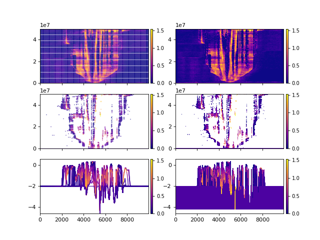
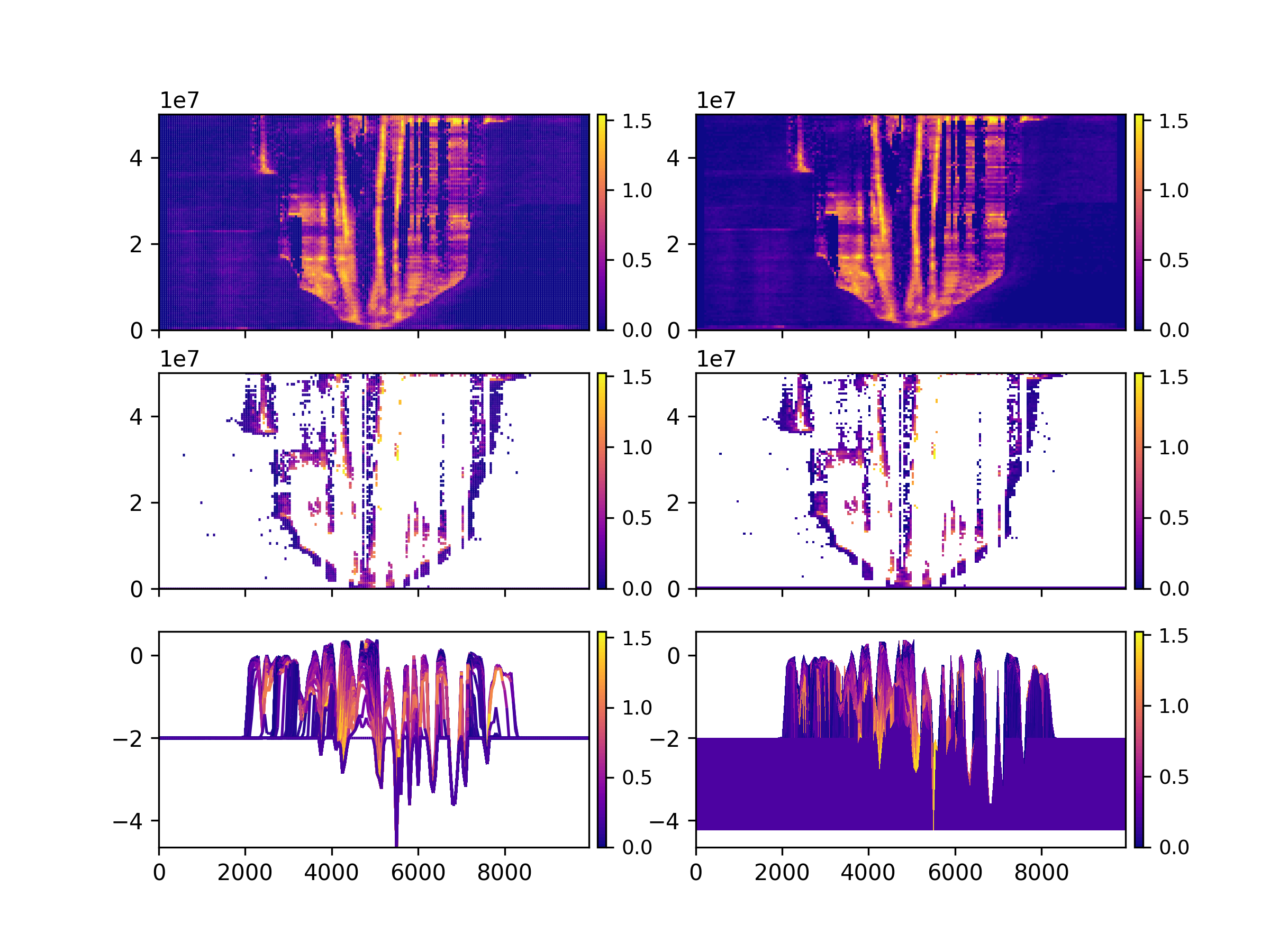
DataCube with computed “quick” stratigraphy may be visualized a number of different ways.

>>> golfcube = spl.sample_data.golf()
>>> golfcube.stratigraphy_from("eta")
>>> golfcube.register_section("demo", spl.section.StrikeSection(distance_idx=10))
>>> _v = "velocity"

>>> fig, ax = plt.subplots(3, 2, sharex=True, figsize=(8, 6))
>>> golfcube.sections["demo"].show(
...     _v, style="lines", data="spacetime", ax=ax[0, 0]
... )
>>> golfcube.sections["demo"].show(
...     _v, style="shaded", data="spacetime", ax=ax[0, 1]
... )
>>> golfcube.sections["demo"].show(
...     _v, style="lines", data="preserved", ax=ax[1, 0]
... )
>>> golfcube.sections["demo"].show(
...     _v, style="shaded", data="preserved", ax=ax[1, 1]
... )
>>> golfcube.sections["demo"].show(
...     _v, style="lines", data="stratigraphy", ax=ax[2, 0]
... )
>>> golfcube.sections["demo"].show(
...     _v, style="shaded", data="stratigraphy", ax=ax[2, 1]
... )
>>> plt.show(block=False)  # doctest +SKIP

(Source code, png, hires.png)